openrowingmonitor/docs/physics_openrowingmonitor.md

The physics behind Open Rowing Monitor

Leading principles

In this model, we try to:

• stay as close to the original data as possible (thus depend on direct measurements as much as possible) instead of depending on derived data. This means that there are two absolute values: time and Number of Impulses;

• use robust calculations as possible (i.e. not depend on a single measurements to reduce effects of measurement errors);

Phases, properties and concepts in the rowing cycle

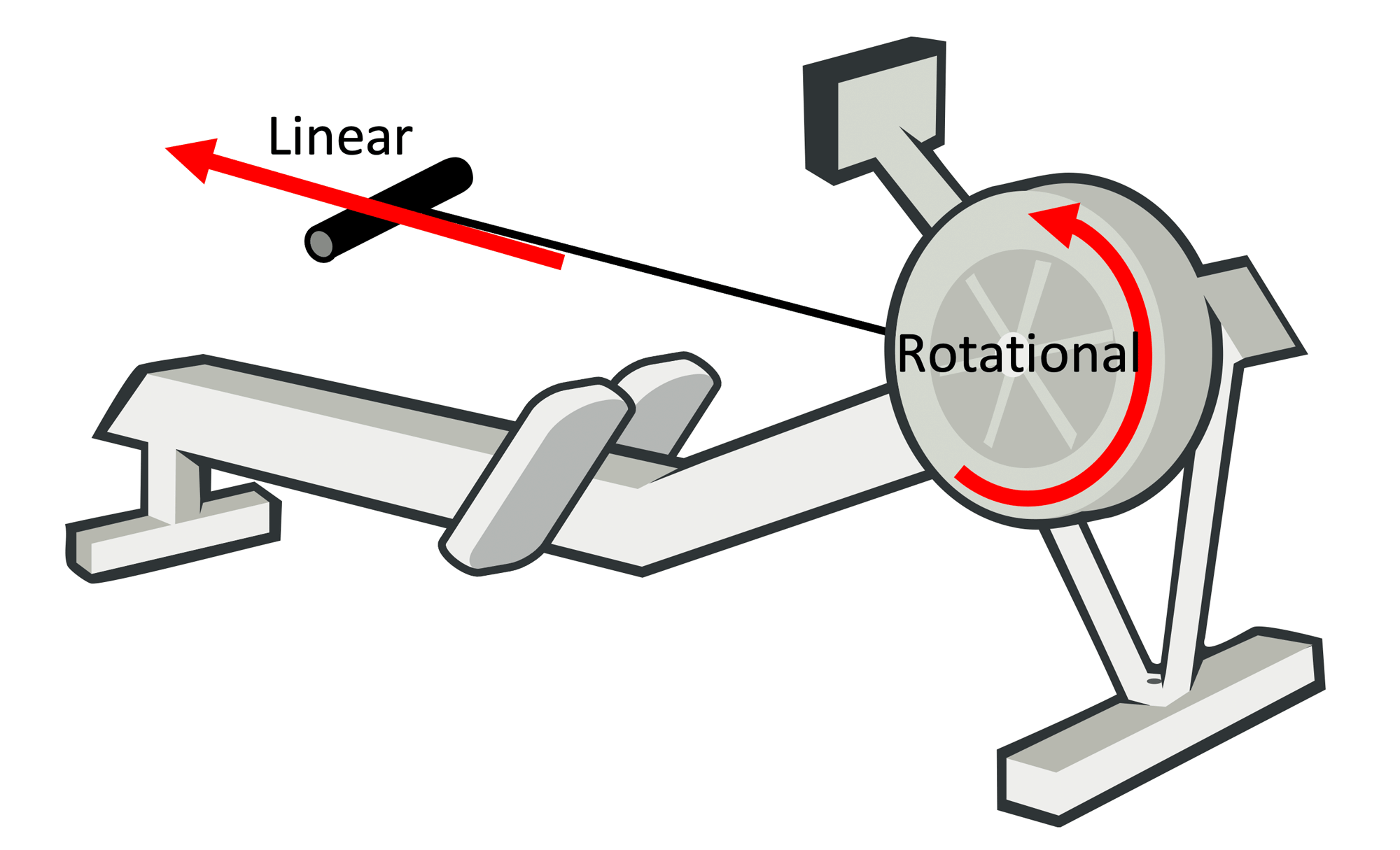
A basic view of an indoor rower

A rowing machine effectively has two fundamental movements: a linear (the rower moving up and down, or a boat moving forward) and a rotational where the energy that the rower inputs in the system is absorbed through a flywheel (either a solid one, or a liquid one).

The linear and rotational speeds are related: the stronger/faster you pull in the linear direction, the faster the flywheel will rotate. The rotation of the flywheel simulates the effect of a boat in the water: after the stroke, the boat will continue to glide, so does the flywheel.

There are several types of rowers:

• Water resistance, where rowing harder will increase the resistance

• Air resistance: where rowing harder will increase the resistance

• Magnetic resistance: where the resistance is constant

Currently, we treat all these rowers as identical as air rowers, although differences are significant.

Typically, measurements are done in the rotational part of the rower, on the flywheel. There is a reed sensor or optical sensor that will measure time between either magnets or reflective stripes, which gives an Impulse each time a magnet or stripe passes. Depending on the number of impulse providers (i.e. the number of magnets or stripes), the number of impulses per rotation increases, increasing the resolution of the measurement. By measuring the time between impulses, deductions about speed and acceleration of the flywheel can be made, and thus the effort of the rower.

Key physical concepts

Here, we distinguish the following concepts:

• The Angular Displacement of the flywheel in Radians: in essence the number of rotations the flywheel has made. As the impulse-givers are evenly spread over the flywheel, the angular displacement between two impulses is 2π/(number of impulse providers);

• The Angular Velocity of the flywheel in Radians/second: in essence the number of rotations of the flywheel per second. As the Angular Displacement is fixed, the Angular Velocity is (angular displacement between impulses) / (time between impulses);

• The Angular Acceleration of the flywheel in Radians/second^2^: the acceleration/deceleration of the flywheel;

• The estimated Linear Distance of the boat in Meters: the distance the boat is expected to travel;

• estimated Linear Velocity of the boat in Meters/Second: the speed at which the boat is expected to travel.

The rowing cycle and detecting the stroke and recovery phase

On an indoor rower, the rowing cycle will always start with a stroke, followed by a recovery. Looking at a stroke, our monitor gets the following data from its sensor:

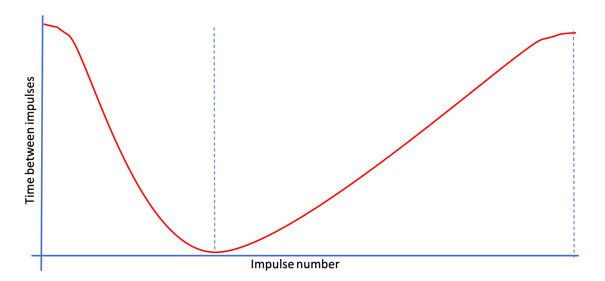
Impulses, impulse lengths and rowing cycle phases

Here, we plot the time between impulses against its sequence number. So, a high number means a long time between impulses, and a low number means that there is a short time between impulses. As this figure also shows, we split the rowing cycle in two distinct phases:

• The Drive phase, where the rower pulls on the handle

• The Recovery Phase, where the rower returns to his starting position

Given that the Angular Displacement between impulses is fixed, we can deduct some things simply from looking at the subsequent time between impulses. When the time between impulses shortens, Angular Velocity is increasing, and thus the flywheel is accelerating (i.e. we are in the drive phase of the rowing cycle). When times between subsequent impulses become longer, the Angular Velocity is decreasing and thus the flywheel is decelerating (i.e. we are the recovery phase of the rowing cycle).

As the rowing cycle always follows this fixed schema, Open Rowing Monitor models it as a finite state machine:

Finite state machine of rowing cycle

Please note: in essence, you can only measure that the flywheel is accelerating/decelerating (thus after it is going on some time), and as we lack the measurement of force on the flywheel, we can't measure the exact moment of acceleration.

Measurements of flywheel

As above picture shows, we can only detect a change in the times between impulses, but where the flywheel exactly accelerates/decelerates is difficult to assess. In essence we only can conclude that an acceleration has taken place somewhere near an impulse, but we can't be certain about where the acceleration exactly takes place. This makes many measurements that depend on this accurate estimate, but not measurements.

Measurements during the recovery phase

Although not the first phase in a cycle, it is an important phase as it deducts specific information about the flywheel properties [1]. During the recovery-phase, we can measure the number of impulses and the length of each impulse. Some things we can easily estimate with a decent accuracy based on the data at the end of the recovery phase:

• The length of time between the start and end of the recovery phase

• The angular displacement between the start and end of the recovery phase

• The angular velocity at the beginning and end of the recovery phase

In the recovery phase, the only force exerted on the flywheel is the (air/water/magnetic)resistance. Thus we can calculate the Drag factor of the Flywheel based on the entire phase.

As [1] describes in formula 7.2:

Or in more readable form:

Looking at the linear speed, we use the following formula [1], formula 9.3:

Or in more readable form:

Looking at the linear speed, we use the following formula [1], formula 9.2:

Or in more readable form:

Measurements during the drive phase

During the drive-phase, we again can measure the number of impulses and the length of each impulse. Some things we can easily estimate with a decent accuracy based on the data at the end of the drive phase:

• The length of time between the start and end of the drive phase

• The angular displacement between the start and end of the drive phase

• The angular velocity at the beginning and end of the drive phase

Looking at the linear speed, we use the following formula [1], formula 9.3:

Or in more readable form:

Looking at the linear speed, we use the following formula [1], formula 9.2:

Or in more readable form:

Power calculation

In the drive phase, the rower also puts a force on the flywheel, making it accelerate.

We can calculate the energy added to the flywheel through [1], formula 8.2:

Or in more readable form for each measured displacement:

Where

The power then becomes

Although this is an easy implementable algorithm by calculating a running sum of this function (see [3], and more specifically [4]). However, the presence of the many Angular Velocities makes the outcome of this calculation quite volatile. The angulate velocity is measured through the formula:

As Time Between Impulses tends to be small (typically much smaller than 1, typically between 0,1 and 0,0015 seconds), small errors tend to increase the Angular Velocity significantly, enlarging the effect of an error and potentially causing this volatility. Currently, this effected is remedied by using a running average on the presentation layer (in RowingStatistics.js). However, when this is bypassed, data shows significant spikes of 20Watts in quite stable cycles due to small changes in the data.

An alternative approach is given by [3], which proposes

Where P is the average power and ω is the average speed during the stroke. Here, the average speed can be determined in a robust manner (i.e. Angular Displacement of the Drive Phase / DriveLength).

As Dave Venrooy indicates this is accurate with a 5% margin. Testing this on live data confirms this behaviour (tested with a autoAdjustDragFactor = true, to maximize noise-effects), with two added observations:

• The simpler measurement is structurally below the more precise measurement when it comes to total power produced in a 30 minutes or 15 minutes row on a RX800 with any damper setting;

• The simpler algorithm is indeed much less volatile: spikes found in the current algorithm are much smaller in the simple algorithm

Following that, I bypassed the running average in the presentation layer and plugged the data in directly. The effects show that the monitor is a bit more responsive but doesn't fluctuate unexpectedly.

As the flywheel inertia is mostly guessed based on its effects on the Power outcome anyway (as nobody is willing to take his rower apart for this), the 5% error wouldn't matter much anyway: the Inertia will simply become 5% more to get to the same power. Using the simpler more robust algorithm has some advantages:

• In essence the instantaneous angular velocities at the flanks are removed from the power measurement, making it more robust against "unexpected" behavior of the rowers (like the cavitation-like effects found in LiquidFlywheel Rowers). Regardless of settings, only instantaneous angular velocities that affect displayed data are the start and begin of each phase;

• Setting autoAdjustDampingConstant to "false" effectively removes/disables all calculations with instantaneous angular velocities (only average velocity is calculated over the entire flank, which typically is not on a single measurement), making Open Rowing Monitor an option for rowers with noisy data or otherwise unstable/unreliable measurements;

• Given the stability of the measurements, it might be an option to remove the filter in the presentation layer completely, making the monitor more responsive to user actions.

Given these advantages and that in practice it won't have a practical implications for users, we think it is best to use the robust implementation.

Additional options and considerations

There are some additional options and considerations:

• Currently, the metrics are only updated at the end of the Recovery Phase, which is once every 2 to 3 seconds. An option would be to update the metrics at the end of the Drive Phase as well.

• An additional alternative would be to update typical end-criteria for trainings that change quite quickly (i.e. absolute distance, elapsed time) every complete rotation;

• Due to reviewing the drag factor at the end of the recovery phase and (retrospectively) applying it to the realized linear distance of that same recovery phase, it would be simpler to report absolute distance from the RowingEngine, instead of added distance;

A closer look at the Drive and Recovery phases

Looking at the average curves of an actual rowing machine, we see the following:

Average curves of a rowing machine

In this graph, we plot the time between impulses (CurrentDt) against the time in the stroke. As CurrentDt is reversely related to angular velocity, we can calculate the angular acceleration/deceleration. In essence, as soon as the acceleration becomes below the 0, the CurrentDt begins to lengthen again (i.e. the flywheel is decelerating). However, from the acceleration/deceleration curve it is also clear that despite the deceleration, there is still a force present: the deceleration-curve hasn't reached its minimum despite crossing 0. This is due to the pull still continuing through the arms: the Netto force is negative due to a part of the arm-moment being weaker than the drag-force of the flywheel. Only approx. 150 ms later the force reaches its stable bottom (and thus the only force is the drag from the flywheel).

Question is if erroneously detecting the recovery-phase too early can affect measurements. The most important measurement here is the calculation of the drag factor. The drag factor can be pinned down if needed by setting autoAdjustDragFactor to "false". If used dynamically, it might affect measurements of both distance and power. In itself the calculation of power is measured based on the power during the drive phase, and thus depends on its correct detection. Distance does not depend directly on phase detection (it just depends on the total number of impulses and the drag factor which is already discussed).

Effects on the drag factor

Our robust implementation of the drag factor is:

Looking at the effect of erroneously starting the recovery early, it affects two variables:

• Recovery length will systematically become too long (approx. 1,5 sec instead of 1,3 sec)

• The Angular Velocity~Start~ will systematically become too high as the flywheel already starts to decelerate at the end of the drive phase, which we mistakenly consider the start of the recovery (approx. 83,2 Rad/sec instead of 82,7 Rad/sec).

Example calculations show that this results in a systematically too high estimate of the drag factor. As these errors are systematic, it is safe to assume these will be fixed by the calibration of the power and distance corrections (i.e. the estimate of the Flywheel Inertia and the MagicConstant).

Effects on the Power calculation

The power calculation is as follows:

Here, the drag factor is affected upwards. Here the average speed is determined by measuring the angular displacement and divided by the time, being affected in the following manner:

• Time spend in the Drive phase is systematically too short

• Angular displacement in the Drive phase will systematically be too short

These effects do not cancel out: in essence the flywheel decelerates at the end of the drive phase, which we mistakenly include in the recovery phase. This means that on average, the average speed is systematically too high: it misses some slower speed at the end of the drive. As all factors of the power calculation are systematically overestimating, the result will be a systematic overestimation.

Again, this is a systematic (overestimation) of the power, which will be systematically corrected by the Inertia setting.

References

[1] Anu Dudhia, "The Physics of ErgoMeters" http://eodg.atm.ox.ac.uk/user/dudhia/rowing/physics/ergometer.html

[2] Marinus van Holst, "Behind the Ergometer Display"

[3] Dave Vernooy, "Open Source Ergometer ErgWare" https://dvernooy.github.io/projects/ergware/

[4] https://github.com/dvernooy/ErgWare/blob/master/v0.5/main/main.ino